Case studyIndependent project
Diabetic retinopathy screening with Grad-CAM
A ResNet-18 transfer-learning model that screens retinal fundus images for diabetic retinopathy, served through a Flask app with a confidence score and a Grad-CAM heatmap, and audited honestly afterwards.
- My role
- Sole developer: data pipeline, training, evaluation, Grad-CAM and Flask app
- Period
- 2025
- Type
- Independent project
The 30-second version
- Problem
- Diabetic retinopathy screening depends on specialists reading fundus photographs; flagging likely cases can help prioritise review, but only if the model is transparent.
- My contribution
- Independent project: I built the training notebook, the evaluation, the Grad-CAM implementation and the Flask app, and later audited my own results.
- Approach
- Frozen ImageNet ResNet-18 with a new two-class head, trained on a public Kaggle dataset with its own train/valid/test split; Grad-CAM via forward and backward hooks.
- Results
- 95.2% accuracy (220/231) on the untouched test set, 91.2% sensitivity, 99.2% specificity, for the final-epoch model. The audit found a checkpoint bug and edge-focused heatmaps.
- Stack
- PyTorch
- torchvision
- ResNet-18
- Grad-CAM
- OpenCV
- Flask
Problem
Diabetic retinopathy damages the blood vessels of the retina and is a leading cause of preventable vision loss. Screening means looking at retinal fundus photographs, and the bottleneck is specialist time. A model that flags likely cases can help prioritise which images a clinician reviews first, but only if it is transparent about why it flagged an image.
Objective
Build a complete, explainable screening prototype: a binary classifier (DR / No DR), an honest evaluation on held-out data, and a web application that returns a prediction, a confidence score and a visual explanation.
Dataset and preprocessing
The model uses the public Diagnosis of Diabetic Retinopathy dataset from Kaggle, which ships with separate training, validation and test folders. Keeping the provided test split untouched until the end is what makes the final number meaningful.
- Images resized to 224 × 224 pixels and normalised with ImageNet statistics, matching the pretrained backbone.
- Random horizontal flips on the training set only; validation and test images are never augmented.
- The held-out test set contains 231 images: 113 DR and 118 No DR, so it is close to balanced.
Architecture
Screening pipeline · select a stage
Stage 1 of 6 · Input
Fundus image upload
A retinal photograph is uploaded through the web app by drag-and-drop or the file picker.
- Animated loading state while the model runs
- Error handling with flash messages
Stage 2 of 6 · Preprocess
Resize and normalise
The image is resized to 224 × 224 and normalised with ImageNet mean and standard deviation, exactly as during training.
- Same transform as validation
- No augmentation at inference
Stage 3 of 6 · Backbone
Frozen ResNet-18
An ImageNet-pretrained ResNet-18 extracts visual features. Its weights are frozen, so only the new head is trained.
- Small enough for CPU inference
- Pretrained features reduce the data needed
Stage 4 of 6 · Head
Classification head
A small fully connected head maps the 512 backbone features to the two classes.
- Linear 512 → 256, ReLU, Dropout 0.3
- Linear 256 → 2 (DR / No DR)
Stage 5 of 6 · Explain
Grad-CAM heatmap
Forward and backward hooks on the last convolution of ResNet-18 produce a class-activation map, overlaid on the input image.
- Shows which regions drove the prediction
- Returned alongside the label
Stage 6 of 6 · Output
Prediction and confidence
The app shows the predicted class, a softmax confidence bar and the Grad-CAM overlay.
- Single request–response cycle in Flask
- Runs on CPU-only machines
Model selection and engineering decisions
- Transfer learning over training from scratch. The dataset is modest in size. A pretrained backbone brings general visual features and makes good accuracy reachable with far less data and compute.
- ResNet-18 rather than a larger network. The goal included a responsive web app on ordinary hardware. ResNet-18 keeps CPU inference fast, and its final convolutional block is a natural Grad-CAM target.
- Freeze the backbone, train only the head. With limited data this lowers the risk of overfitting and makes training quick and stable. The trade-off is that the features are never adapted to retinal images, which caps achievable accuracy.
Training and evaluation
Training used cross-entropy loss and Adam (learning rate 0.001) on the head parameters, batch size 32, for 20 epochs, tracking validation accuracy every epoch.
Accuracy per epoch
Loss per epoch
View data table
| Epoch | Train loss | Train acc | Val loss | Val acc |
|---|---|---|---|---|
| 1 | 0.2752 | 89.16% | 0.1474 | 94.35% |
| 2 | 0.1867 | 93.45% | 0.1556 | 93.60% |
| 3 | 0.1527 | 94.99% | 0.1225 | 95.48% |
| 4 | 0.1454 | 95.47% | 0.1186 | 95.10% |
| 5 | 0.1485 | 94.89% | 0.1533 | 94.16% |
| 6 | 0.1941 | 93.11% | 0.1180 | 95.67% |
| 7 | 0.1349 | 95.66% | 0.1105 | 96.23% |
| 8 | 0.1392 | 95.47% | 0.1191 | 95.86% |
| 9 | 0.1238 | 95.86% | 0.1023 | 96.23% |
| 10 | 0.1245 | 95.91% | 0.1779 | 93.79% |
| 11 | 0.1269 | 95.52% | 0.1064 | 96.05% |
| 12 | 0.1227 | 96.00% | 0.1823 | 93.03% |
| 13 | 0.1245 | 95.81% | 0.1081 | 96.05% |
| 14 | 0.1430 | 94.75% | 0.1135 | 95.67% |
| 15 | 0.1260 | 95.76% | 0.1121 | 96.05% |
| 16 | 0.1113 | 96.05% | 0.1039 | 96.61% |
| 17 | 0.0927 | 97.16% | 0.0956 | 96.99% |
| 18 | 0.0977 | 97.11% | 0.1161 | 96.42% |
| 19 | 0.0966 | 96.68% | 0.1163 | 96.23% |
| 20 | 0.1103 | 96.00% | 0.1795 | 93.79% |
The checkpoint bug, and what the 95.2% really represents
The loop was meant to remember the best-validation weights and restore them before testing. This is the code, verbatim:
if phase == 'valid' and epoch_acc > best_acc:
    best_acc = epoch_acc
    best_model_wts = model.state_dict()
...
model.load_state_dict(best_model_wts)
state_dict() returns references to the model’s live tensors, not copies. Every later optimiser step (and every BatchNorm statistics update in training mode) changes the “snapshot” too, so load_state_dict(best_model_wts) restores the weights the model already has. The model evaluated on the test set is the final, epoch-20 model, whose validation accuracy was 93.79%, not the epoch-17 model at 96.99%. The 95.2% test accuracy is a genuine measurement of that final model; the epoch-17 model was never tested, so I do not claim anything about it.
The fix is one line, best_model_wts = copy.deepcopy(model.state_dict()), or saving a checkpoint file at the best epoch. It has not yet been applied and re-run; the full story is in The checkpoint bug that changed my reported model.
Results
- Test accuracy
- 95.2%
- 220 of 231
- Sensitivity (DR recall)
- 91.2%
- 103 of 113
- Specificity
- 99.2%
- 117 of 118
- Test images
- 231
- held out
- Accuracy
- 95.2%
- 220 / 231
- Sensitivity (DR recall)
- 91.2%
- 103 / 113
- Specificity
- 99.2%
- 117 / 118
- Precision (DR)
- 99.0%
- 103 / 104
What each cell means
- True positive · 103
- 103 images with DR that the model flagged as DR.
- False negative · 10
- 10 images with DR that the model labelled No DR: missed cases, the costly error in screening.
- False positive · 1
- 1 image without DR that the model flagged as DR: a false alarm.
- True negative · 117
- 117 images without DR that the model correctly labelled No DR.
If the same rates held at another prevalence
Illustrative arithmeticThis test set: 48.9% (113 of 231)
- Precision (a positive flag is right)
- 92.3%
- Negative predictive value
- 99.0%
Per 10,000 screened: about 912 correctly flagged, 88 missed, 76 false alarms.
Formulas and assumptions
Measured on this test set: sensitivity = 103 / 113 = 91.2%; specificity = 117 / 118 = 99.2%. With assumed prevalence p:
This assumes the measured rates stay the same at other prevalences, which is an assumption, not a measurement. They come from one test set of 231 images, are not clinical performance or validated screening results, and say nothing about how the model would behave on other populations or cameras.
| Prevalence | Precision | NPV |
|---|---|---|
| 1.0% | 52.1% | 99.9% |
| 5.0% | 85.0% | 99.5% |
| 10.0% | 92.3% | 99.0% |
| 20.0% | 96.4% | 97.8% |
| 48.9% (test set) | 99.0% | 92.1% |
The model is conservative: it almost never raises a false alarm (1 of 118 healthy images), but it misses 10 of 113 DR cases. For screening, a missed case costs more than a false alarm, so the next version should trade some specificity for sensitivity, for example by tuning the decision threshold on the validation set.
Explainability
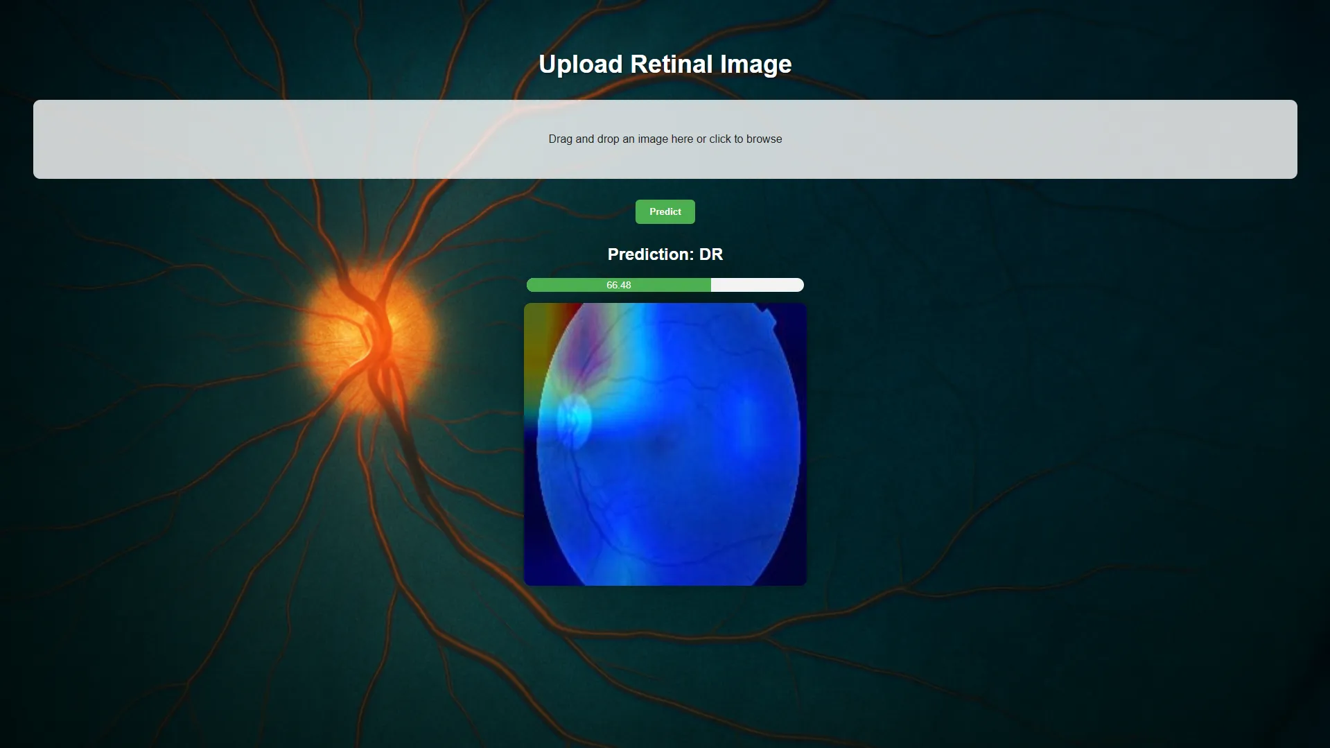
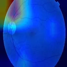
Before reading these images, it helps to know how they were drawn. The overlay code in model/model.py is:
heatmap = cv2.applyColorMap(cam, cv2.COLORMAP_JET)
superimposed = heatmap * 0.4 + orig

gradcam_path = "static/gradcam.jpg"
cv2.imwrite(gradcam_path, superimposed)
applyColorMap returns BGR and cv2.imwrite expects BGR, so the heatmap colours are correct (red and yellow mean high activation). But orig comes from PIL in RGB order, so the retina’s own colours are swapped: the orange fundus is rendered blue. The sum is also not clipped before saving, which washes out bright areas.
With that in mind, the reading is clear: in the saved output (the same image appears in both figures above), the hottest region sits at the edge of the fundus, not on lesions such as haemorrhages or exudates. A correct label with an explanation pointing at the border can mean the model has learned a shortcut, such as the edge of the camera’s field of view. One image is not a systematic audit, so I treat this as a warning sign rather than a conclusion. The broader discussion is in What Grad-CAM revealed about shortcut learning.
Application workflow
The Flask application wraps the trained model in a single request–response flow: upload, validate, preprocess, predict, compute Grad-CAM, render. The front end provides drag-and-drop upload, a loading state, an animated confidence bar and readable error messages. Inference runs on the CPU.
Challenges, trade-offs and lessons
- Trusting a variable name.
best_model_wtssounded right, so the restore step was never verified. A one-line assertion that the restored weights differ from the final weights would have caught it. - Accuracy hides the costly error. Publishing the confusion matrix makes the 10 missed DR cases visible instead of burying them in 95.2%.
- Visualisation code is part of the model’s credibility. A channel-order slip changes what a reader sees. Explanations need the same review as metrics.
- Speed versus adaptation. Freezing the backbone made training fast and stable but limits how well the model fits retinal images.
What I would do next
- Fix the checkpoint copy, re-run, and report the best-validation model alongside the final one.
- Fine-tune the last ResNet block, not only the head.
- Tune the decision threshold for sensitivity and report the ROC curve.
- Fix the overlay colour order and clipping, then audit Grad-CAM across the whole test set (for example, the share of activation inside the fundus versus at its edge).
- Validate on a second, independent fundus dataset.
Repository
The code, notebook and Flask app are on GitHub.
Related writing
The checkpoint bug that changed my reported model
My diabetic retinopathy model reported 95.2% test accuracy, and the notebook said it came from the best-validation epoch. One missing copy meant it did not. What happened, how I found it, and what the number really means.
Read articleWhat Grad-CAM revealed about shortcut learning
Explanation methods are meant to show whether a model looks at the right place. In two medical-imaging projects they raised real questions about my models, and once, through a colour bug, nearly pointed me to the wrong conclusion.
Read article