Both of my medical-imaging projects return a visual explanation with every prediction. I added them so that a clinician could see why a model made a call. In practice, the most valuable thing the explanations did was make me question the models, and in one case, question my own reading of the explanations.
Two explanation methods in one paragraph each
Grad-CAM takes the gradient of the predicted class score with respect to the last convolutional feature maps, averages each map’s gradient into a weight, and sums the maps with those weights. After a ReLU and upsampling to the image size, bright regions are those that pushed the prediction up. It is fast and tied to the network’s internals, but coarse: for ResNet-style networks at 224 px the map starts at 7 × 7 and is stretched over the whole image.
LIME treats the model as a black box. It splits the image into superpixels, switches random subsets off, records how the prediction changes, and fits a simple linear model to those perturbations. Superpixels with positive weights support the prediction. It works the same way for any model, but its output depends on sampling and segmentation choices, so it can be noisy.
How Grad-CAM works
From one prediction to a heatmap, in seven steps
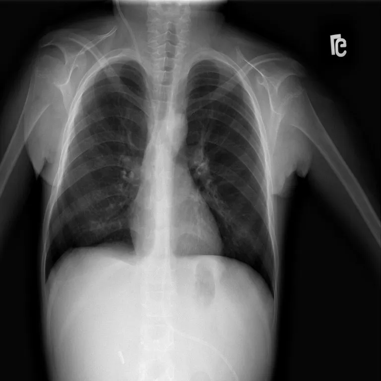
Steps 1 and 7 are a real LungVision scan and the Grad-CAM the app saved for it. Steps 2–6 are schematic illustrations with made-up values, not recorded activations of the trained models.
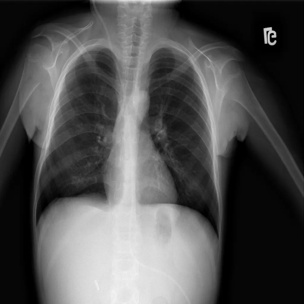 Real input
01 · Input
An image goes in
The model classifies the scan as usual. Grad-CAM asks a follow-up question: which regions pushed the score for the predicted class up?
- Schematic · not recorded activations
02 · Last convolutional layer
Take the final feature maps
Grad-CAM looks at the last convolutional layer, whose feature maps still keep a coarse spatial layout of the image. Each map responds to some learned pattern.
- Schematic · not recorded activations
03 · Gradients → weights
Weigh each map by its gradient
The gradient of the class score with respect to each feature map, averaged over its positions, says how much that channel mattered for this prediction.
- Schematic · not recorded activations
04 · Weighted combination
Add the weighted maps together
Multiplying each map by its weight and summing gives one coarse map. It can contain negative regions: evidence against the class.
- Schematic · not recorded activations
05 · ReLU
Keep only positive evidence
A ReLU sets the negative values to zero, so the map only shows regions that supported the predicted class.
- Schematic · not recorded activations
06 · Upsample and normalise
Resize and scale to 0–1
The coarse map is resized to the input image and scaled to between 0 and 1, ready to be coloured with a colour map such as JET.
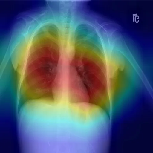 Real saved output · model C
07 · Overlay
Blend it over the scan
The coloured map is blended over the original image. It shows where the model looked for this class, not whether it was right, and not why.
What shortcut learning looks like
A model learns a shortcut when it finds a feature that predicts the label in the training data but has nothing to do with the task. In chest radiography this is well documented: Zech et al. (PLOS Medicine, 2018) showed pneumonia models that performed worse at hospitals they had not seen and could recognise which hospital an image came from, and DeGrave, Janizek and Lee (Nature Machine Intelligence, 2021) showed COVID-19 detectors relying on confounders such as text markers and patient positioning rather than lung pathology. Accuracy alone cannot reveal this. Explanations sometimes can.
Case 1: a retina model looking at the edge
The diabetic retinopathy app saves one Grad-CAM overlay in its repository. In it, the hottest region sits at the edge of the fundus, the boundary of the camera’s circular field of view, rather than on lesions such as haemorrhages or exudates.
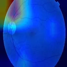
Reading this correctly required reading the code first. The overlay adds an OpenCV colour map (BGR) to a PIL image (RGB) and writes the result with OpenCV, which expects BGR. The heatmap therefore keeps its true colours, while the orange retina is rendered blue. Once that is clear, the observation stands: on this example, the strongest evidence for “DR” lies at the border. One image is not an audit, but it is exactly the pattern a shortcut would produce.
Case 2: LungVision, and a reading I had to reverse
LungVision runs four CNNs per scan and saves a Grad-CAM and a LIME explanation for each. The repository keeps hundreds of these outputs, with different random file names for the upload and its explanations. To study them properly I first matched each explanation to its original scan by correlating fine image detail (the smooth heatmap contributes almost nothing to it), which recovered 30 complete sets: each original with all four of its Grad-CAMs and its LIME outputs, matching far more strongly than any other image.
The first reading of those heatmaps, made while preparing this write-up, was alarming: warm colours along the image borders, cool blue inside the lungs. It looked like a textbook shortcut. Then I read the overlay function:
heatmap_colored = cv2.applyColorMap(heatmap_normalized, cv2.COLORMAP_JET)
overlay = cv2.addWeighted(img, 0.6, heatmap_colored, 0.4, 0)
applyColorMap returns BGR; img is RGB. The blend mixes channel orders, and after saving, red and blue are swapped: blue means high attention. Because chest X-rays are greyscale, swapping the two channels back reproduces the correctly coloured overlay exactly.
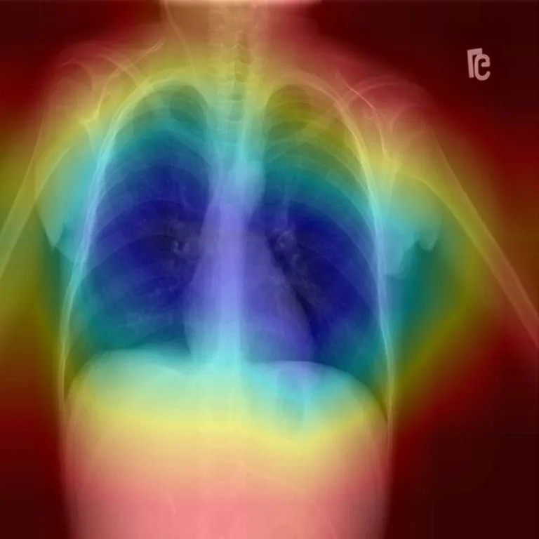
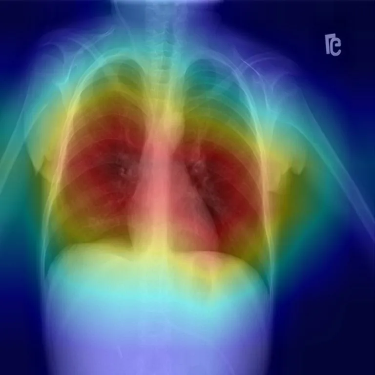
Corrected, the picture is different. The four networks attend mostly to the chest, though each to a different region, which the averaged prediction hides. Read properly, Grad-CAM is more reassuring, with the usual caveat: it shows where a model looked, not whether it was right.
LIME: four runs, four different answers
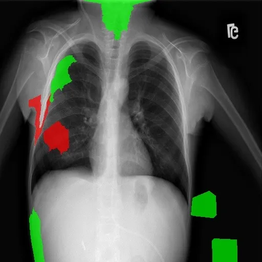
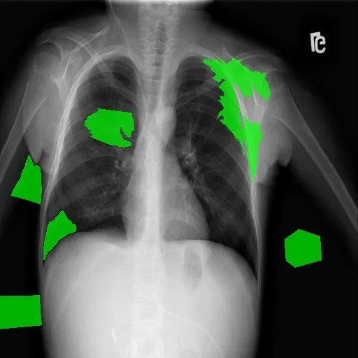
The app also saved four LIME outputs for this scan, one per model run. An earlier version of this write-up compared the Grad-CAM above with a single LIME output that pointed at the shoulder and abdomen, and treated the difference as “Grad-CAM versus LIME”. That comparison does not hold up. Here are all four runs:
 Run 1
 Run 2
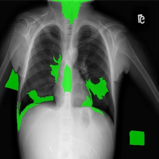 Run 3
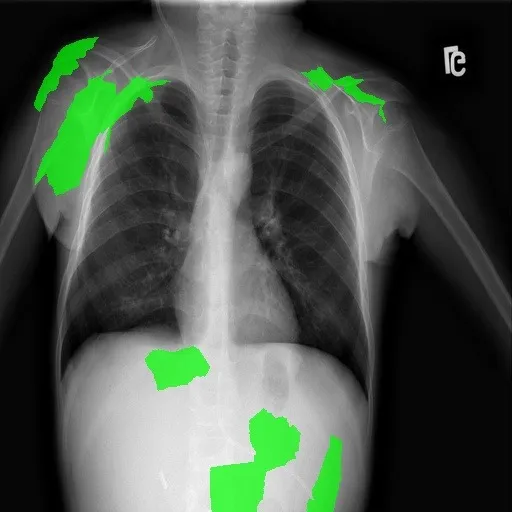 Run 4
They barely agree. Some runs place supporting superpixels inside the lung fields; others place them on the shoulders, the image edge, below the diaphragm or outside the body. To check whether this scan was unusual, I measured the overlap of supporting regions across every matched scan: for each scan, the intersection-over-union (IoU) of the green regions for each pair of runs. Across 30 scans and 180 pairs, the median IoU was 0.00 (interquartile range 0.00–0.06, maximum 0.25); 99% of pairs overlapped by less than 0.2.
Two limits matter here. First, the app runs LIME once per ensemble model and does not record which file belongs to which model, so the variation mixes genuine differences between models with LIME’s own random sampling, and no LIME run can be paired with a specific Grad-CAM. Second, the supporting regions were extracted by colour from the saved images (green clearly dominating red and blue), which is reliable for the app’s flat green fills but is a measurement of the saved pictures, not of LIME’s internal weights.
So the honest finding is not that one method disagrees with another. It is that these LIME explanations are too unstable to support conclusions on their own. The off-lung regions that appear in some runs are still worth taking seriously as a prompt to test for shortcut learning, but they are not evidence of it.
What a proper check would look like
I have not run these yet. They are the next step, and they turn impressions into numbers:
- Stable explanations first. Repeat LIME several times per model with recorded seeds and model names, and report how much the runs agree before interpreting any of them.
- Attribution inside a lung mask. Segment the lung fields and measure what share of the Grad-CAM and LIME attribution falls inside them, across the whole test set rather than a few images.
- Occlusion tests. Mask the borders and side markers and check whether predictions change; then mask the lungs and check whether they don’t change. A model that ignores lungs but reacts to markers is using a shortcut.
- Crop before classifying. Train on cropped or segmented lung fields so off-lung features are unavailable, and compare.
- External validation. Evaluate on images from a different source, where source-specific cues no longer line up with labels.
What I learned
- Visualisation code is part of the model. A one-line channel-order slip inverted every LungVision heatmap. Explanations deserve the same code review as training and evaluation.
- Check stability before meaning. A single LIME run looked like a clear story; four runs showed it was mostly noise. Explanations need repeated runs and a measure of agreement, just like metrics need confidence intervals.
- Do not pair outputs you cannot link. Without a record of which explanation came from which model, side-by-side comparisons can quietly mix models and methods.
- Quantify before concluding. A gallery of examples is a hypothesis generator, not evidence.
- Say what you have not done. The interesting part of this story is the open question, and it should be labelled as one.
The projects themselves are described in the LungVision and diabetic retinopathy case studies.